TopMSV
In this tutorial, we show how to install and start TopMSV and how to use it to visualize an example top-down LC-MS/MS dataset that has been processed by TopFD and TopPIC. A description of every page and its operations is given on the manual page.
1. Installing Node.js (Linux and macOS only)
TopMSV runs on Node.js version 24 or newer. On Windows, this step can be skipped because the Windows zip file of TopMSV includes Node.js. On Linux and macOS, an easy way to install Node.js is nvm (Node Version Manager).
- Install nvm by
running the following command in a terminal, and then restart the
terminal.
curl -o- https://raw.githubusercontent.com/nvm-sh/nvm/v0.40.3/install.sh | bash
- Install Node.js 24 with the following commands. The last command
should print a version starting with
v24.nvm install 24 nvm use 24 node -v
2. Downloading TopMSV
- Go to the Download page.
- Choose the download type "Windows zip file" or "Linux". The Windows zip file contains TopMSV together with Node.js, all its dependencies, and the compiled browser scripts. The Linux option opens the release page of TopMSV on GitHub, where the source code archive can be downloaded.
- Fill out the registration form and click "I accept the license agreement and download TopMSV".
- Unzip the downloaded archive to a folder, for example
C:\topmsvon Windows or~/topmsvon Linux and macOS. The folder contains the filepackage.jsonand, on Windows, the batch filestart_server.bat.
3. Starting the TopMSV server
3.1 Windows
Double-click the batch file start_server.bat in the
TopMSV folder. The script starts the server at
http://localhost:3000; no installation or build step is
needed because the zip file already contains Node.js, the dependencies,
and the browser scripts. Keep the terminal window open while TopMSV is
used, and press Ctrl+C in it to stop the server.
3.2 Linux and macOS
Open a terminal in the TopMSV folder and run the following commands.
The first two commands are needed only once after the download: they
install the dependencies and build the browser scripts. The last
command starts the server at http://localhost:3000; press
Ctrl+C to stop it.
npm install
npm run build:client
npm start
3.3 Options
The port and the directory in which uploaded datasets are stored can
be changed with the environment variables PORT and
DATA_DIR. By default, datasets are stored in the folder
data inside the TopMSV folder. For example, the following
command starts the server at port 8080 with datasets stored in
/path/to/data:
DATA_DIR=/path/to/data PORT=8080 npm start
On Windows, set the variables in the terminal before running the
batch file, for example set PORT=8080. To share existing
datasets without allowing uploads or deletions, start a read-only
server with the option --view-only:
npm start -- --view-only
On Windows, run start_server.bat --view-only from a
terminal instead.
4. Example dataset
In the MS experiment, the protein extract of S. typhimurium was reduced with dithiothreitol and alkylated with iodoacetamide. The protein mixture was first separated by gas-phase fractionation, resulting in 7 fractions. Each fraction was separated by an HPLC system coupled to an LTQ-Orbitrap mass spectrometer (Thermo Fisher Scientific). MS and MS/MS spectra were collected at a resolution of 60,000 and 30,000, respectively. In this tutorial, we use only the LC-MS/MS data file of the first fraction.
The data file was deconvoluted with TopFD, and the deconvoluted
spectra were searched against the S. typhimurium proteome database
from UniProt with TopPIC. Both tools are available at
toppic.org. TopFD wrote the
deconvoluted spectra and the MS1 3D peak tables into the SQLite file
st_1.sqlite, and TopPIC appended its identifications and
the protein database to the same file, so the whole dataset is one
file.
- Download the example archive topmsv_data.zip (about 210 MB).
- Unzip the archive to obtain the file
st_1.sqlite(about 540 MB), for example in the folderC:\topmsv_dataon Windows or~/topmsv_dataon Linux and macOS.
5. Uploading the dataset
- Open a web browser and go to
http://localhost:3000to show the home page of TopMSV. - In the panel "Upload a dataset", type
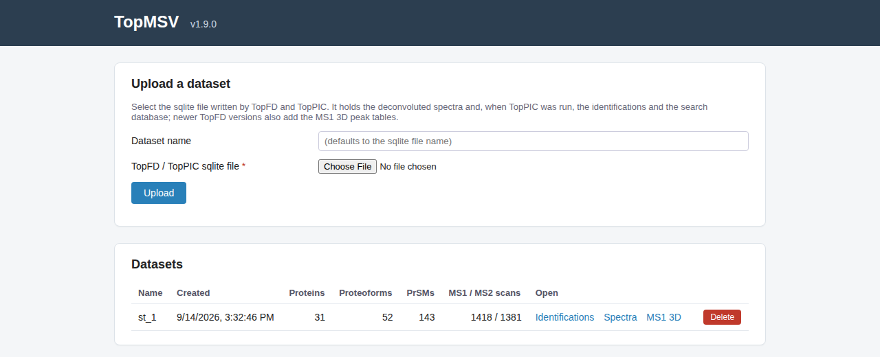
st_1as the dataset name (optional; the file name is used when it is left empty), click "Choose File" to select the filest_1.sqlite, and click "Upload". The upload of the file takes a moment. When the upload is finished, the message "Dataset "st_1" is ready." is shown and the dataset appears in the "Datasets" table. - The table shows that the dataset has 31 identified proteins, 52 proteoforms, 143 PrSMs (proteoform-spectrum-matches), 1418 MS1 scans, and 1381 MS/MS scans, and it has three links: "Identifications", "Spectra", and "MS1 3D". A dataset is removed from the server with the "Delete" button.
6. Data visualization
6.1 Protein identifications
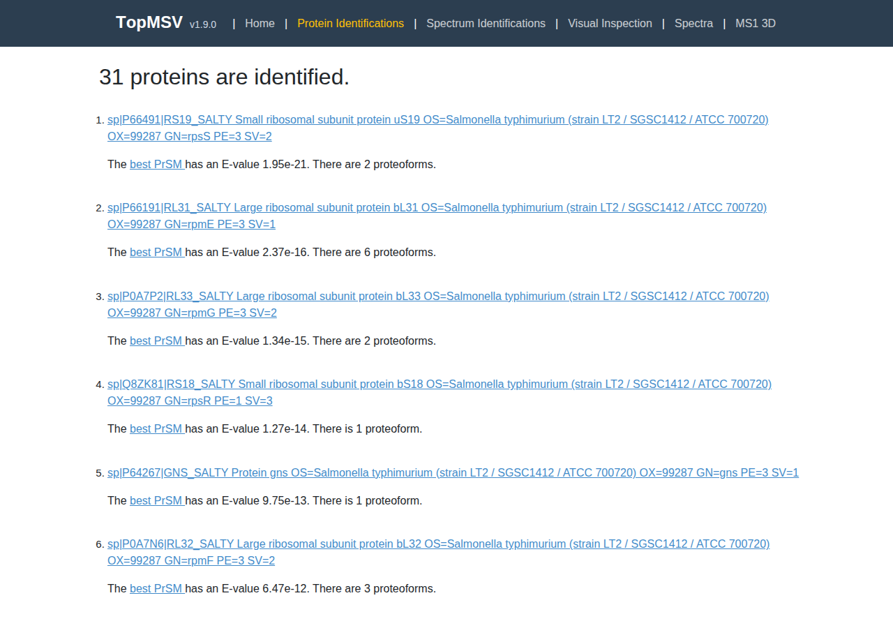
- Click "Identifications" in the "Datasets" table (or "Protein Identifications" in the navigation bar of any dataset page). The page lists the 31 identified proteins with the E-value of the best PrSM and the number of proteoforms of each protein.
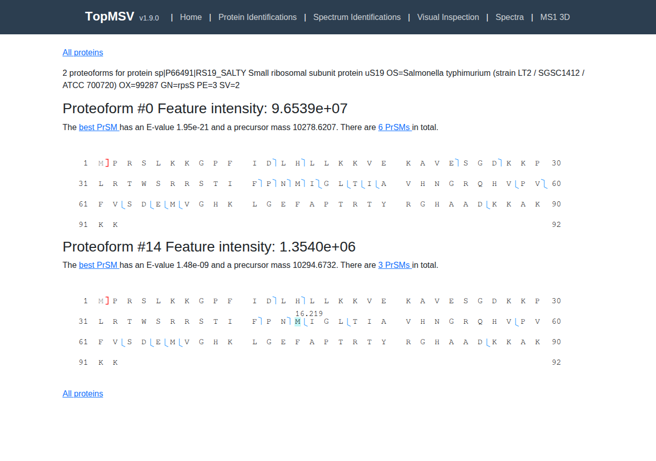
- Click the first protein, the small ribosomal subunit protein uS19 (sp|P66491|RS19_SALTY). The protein page shows its two identified proteoforms with their annotated sequences. Proteoform #14 carries an unexpected mass shift of 16.219 Da, drawn above the shifted residue.
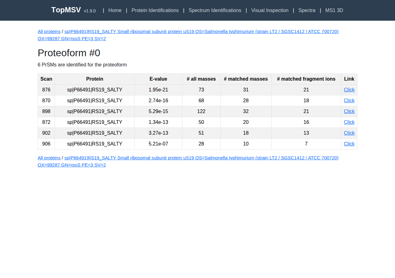
- Click the link "6 PrSMs" of Proteoform #0. The proteoform page lists the six PrSMs of the proteoform with their scan numbers, E-values, and numbers of matched masses and fragment ions.
- Click "Click" in the first row (scan 876) to open the PrSM page.
6.2 Inspecting a PrSM
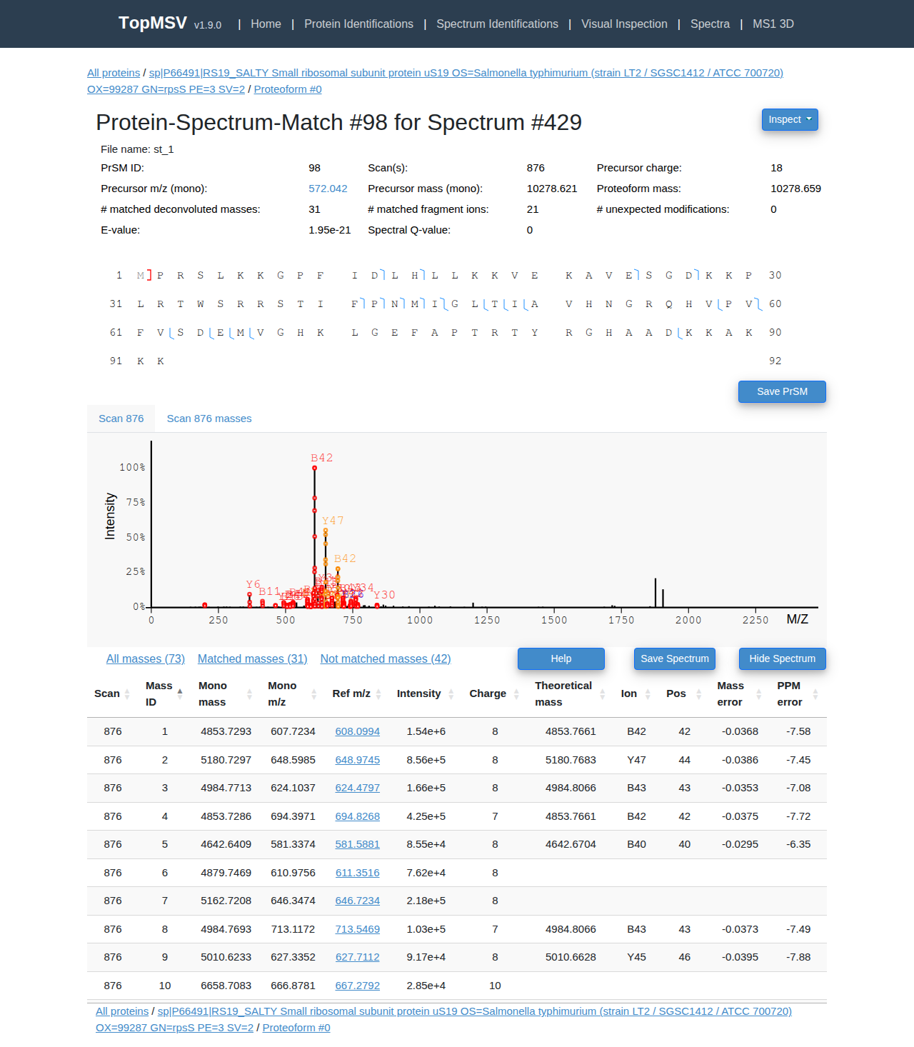
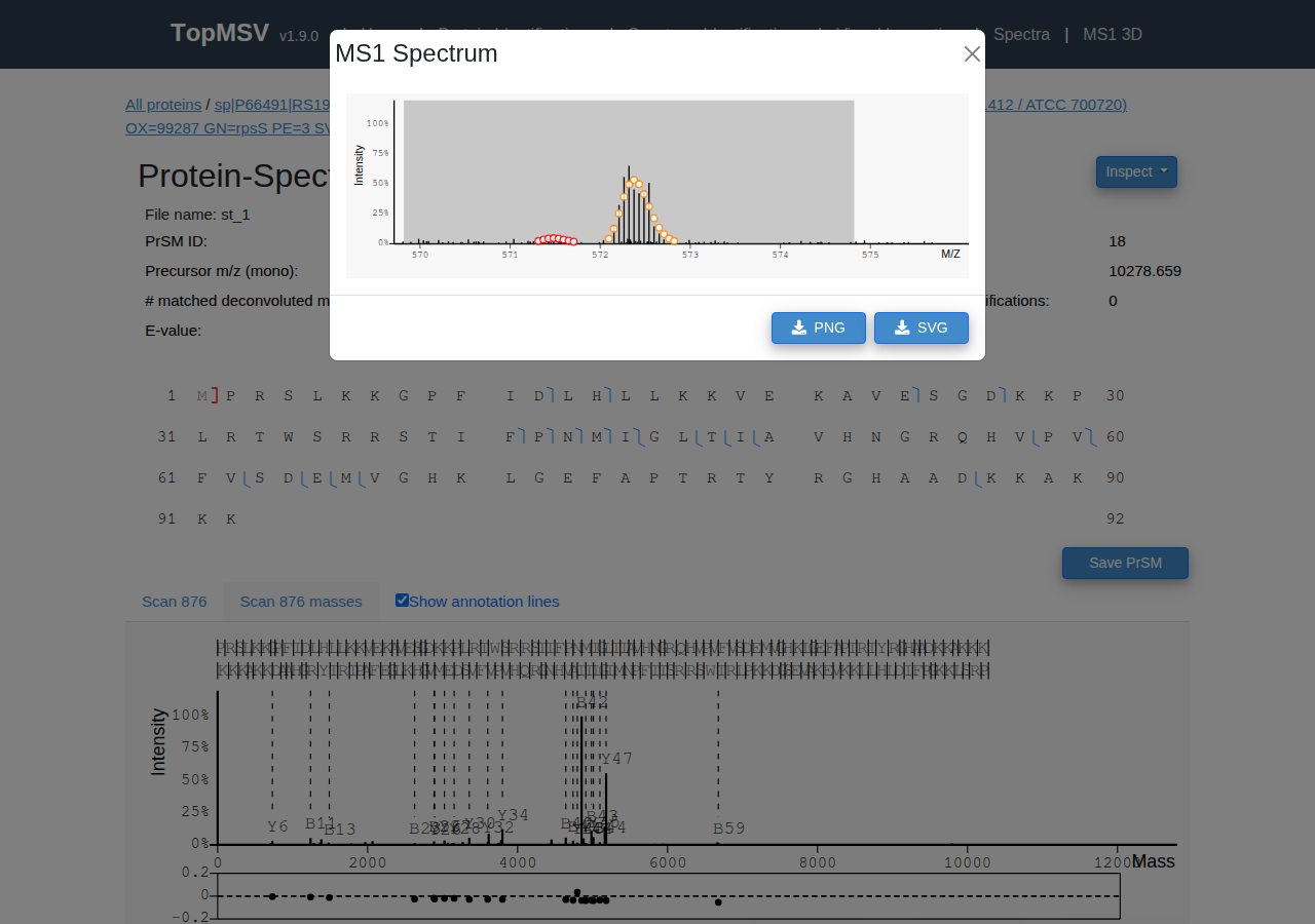
- The PrSM page shows a summary table of the match, the annotated proteoform sequence, and a table of the deconvoluted masses of the MS/MS spectrum. Hover over a blue bracket in the sequence to see the fragment ions matched at the cleavage site, and click a bracket to filter the mass table to those ions.
- Click "Show Spectrum" to show the MS/MS spectrum. Circles mark the peaks of the isotopic envelopes reported by TopFD, and matched envelopes are labeled with their ion names. Drag the spectrum with the mouse, and use the mouse wheel below the x axis to zoom the m/z range or above the x axis to scale the intensities.
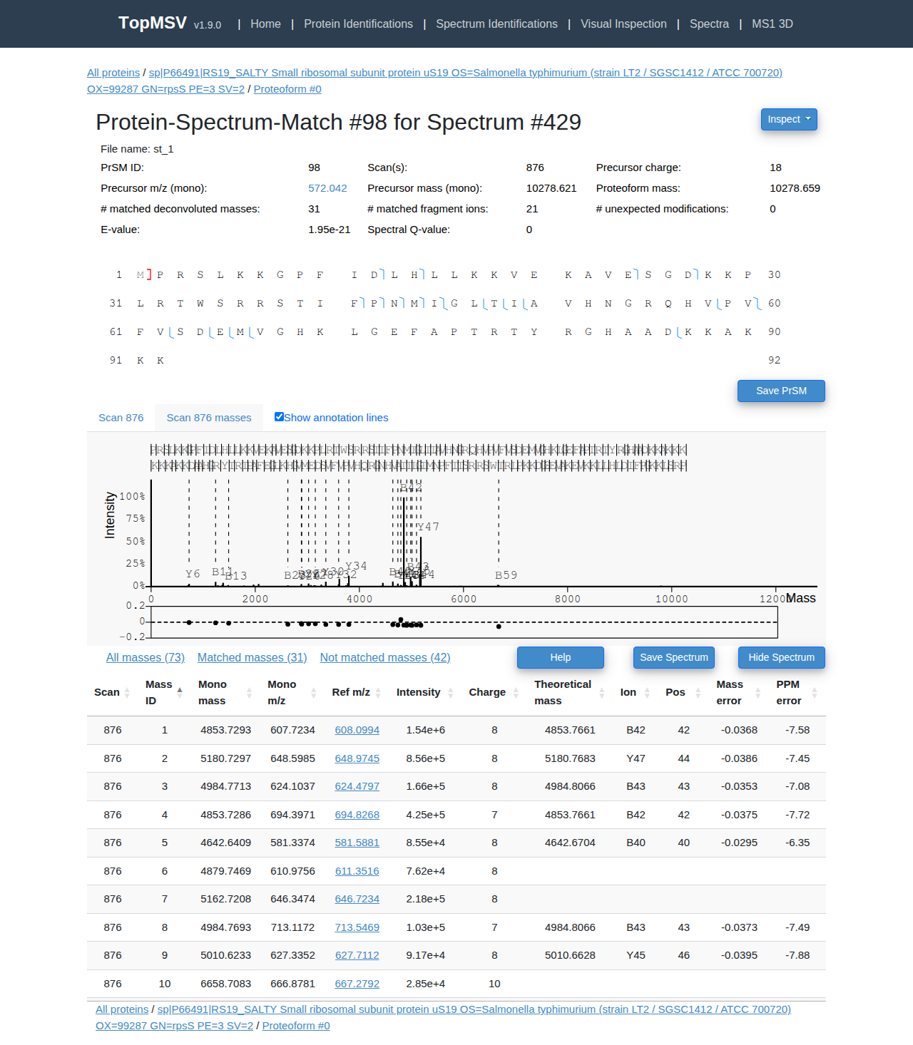
- Click the tab "Scan 876 masses" to show the deconvoluted masses together with the theoretical fragment masses of the proteoform and an error plot of the matched masses.
- Click the precursor m/z value 572.042 in the summary table to open a popup window with the MS1 spectrum, in which the isolation window of the precursor is highlighted.
- Click a value in the "Ref m/z" column of the mass table to center the MS/MS spectrum at the envelope. Use the links "All masses", "Matched masses", and "Not matched masses" to filter the table.
- Click "Save PrSM" to save the annotated sequence as an image, and "Save Spectrum" to save the spectrum view.
6.3 Visual inspection
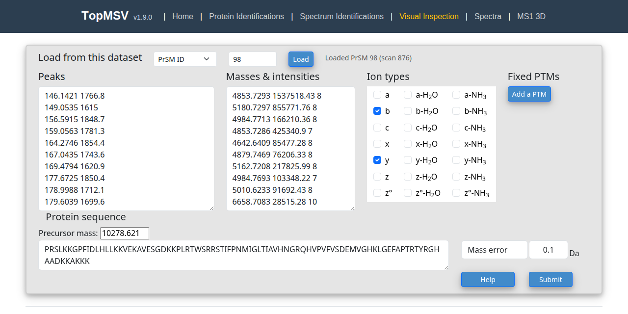
- On the PrSM page, click the "Inspect" button at the top right and
choose "Scan 876". The visual inspection page opens in a new tab
with the peaks, deconvoluted masses, ion types, protein sequence, and
precursor mass of the PrSM filled in. The same page can be opened
from the navigation bar; in that case, choose "PrSM ID" in the
"Load from this dataset" dropdown, type
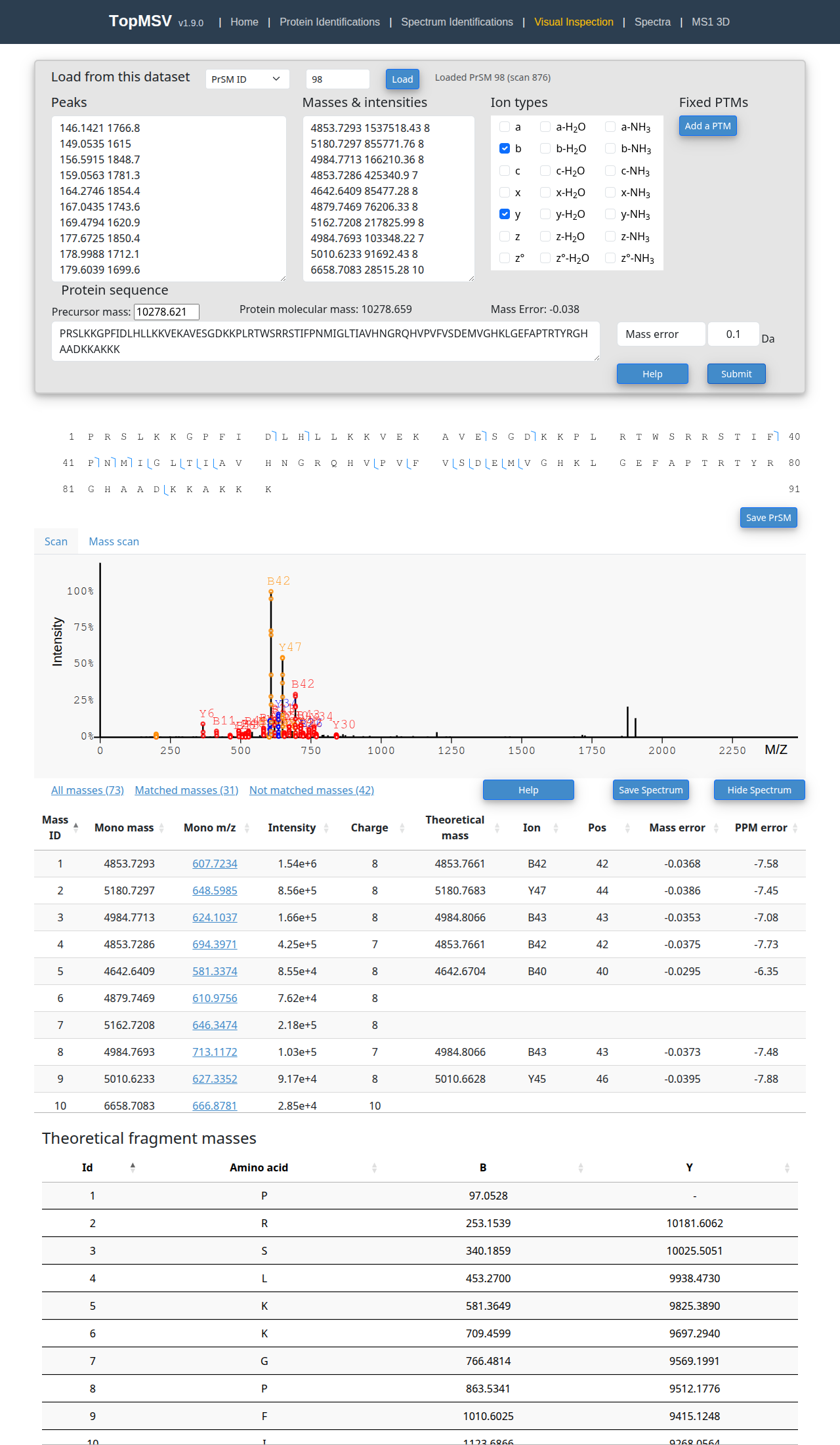
98, and click "Load". - Click "Submit". The annotated sequence, the MS/MS spectrum, the mass table, and a table of theoretical fragment masses are shown.
- The inputs can be edited to test alternative explanations of the spectrum. For example, select additional ion types, change the error tolerance to "PPM error", or edit the protein sequence, and click "Submit" again. Click a residue in the annotated sequence to add a variable PTM or an unknown mass shift at the residue.
6.4 Spectra browser
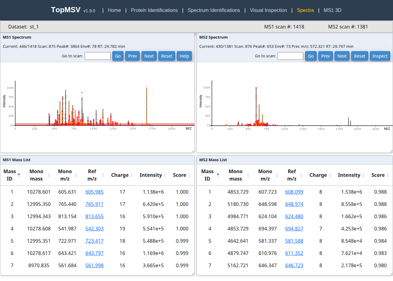
- Click "Spectra" in the navigation bar. The page shows the first MS1 and MS/MS scans of the dataset with their envelopes in the mass lists.
- In the "MS2 Spectrum" panel, type
876in the "Go to scan" box and click "Go". The MS/MS scan 876 is shown, and its precursor MS1 scan 875 is shown automatically in the "MS1 Spectrum" panel. Use "Prev" and "Next" to move between scans. - Click a circle in a spectrum to highlight the envelope in the mass list, and click a "Ref m/z" value in a mass list to center the spectrum at the envelope.
- Click "Inspect" in the "MS2 Spectrum" panel to open the current MS/MS spectrum in the visual inspection page.
6.5 MS1 3D view
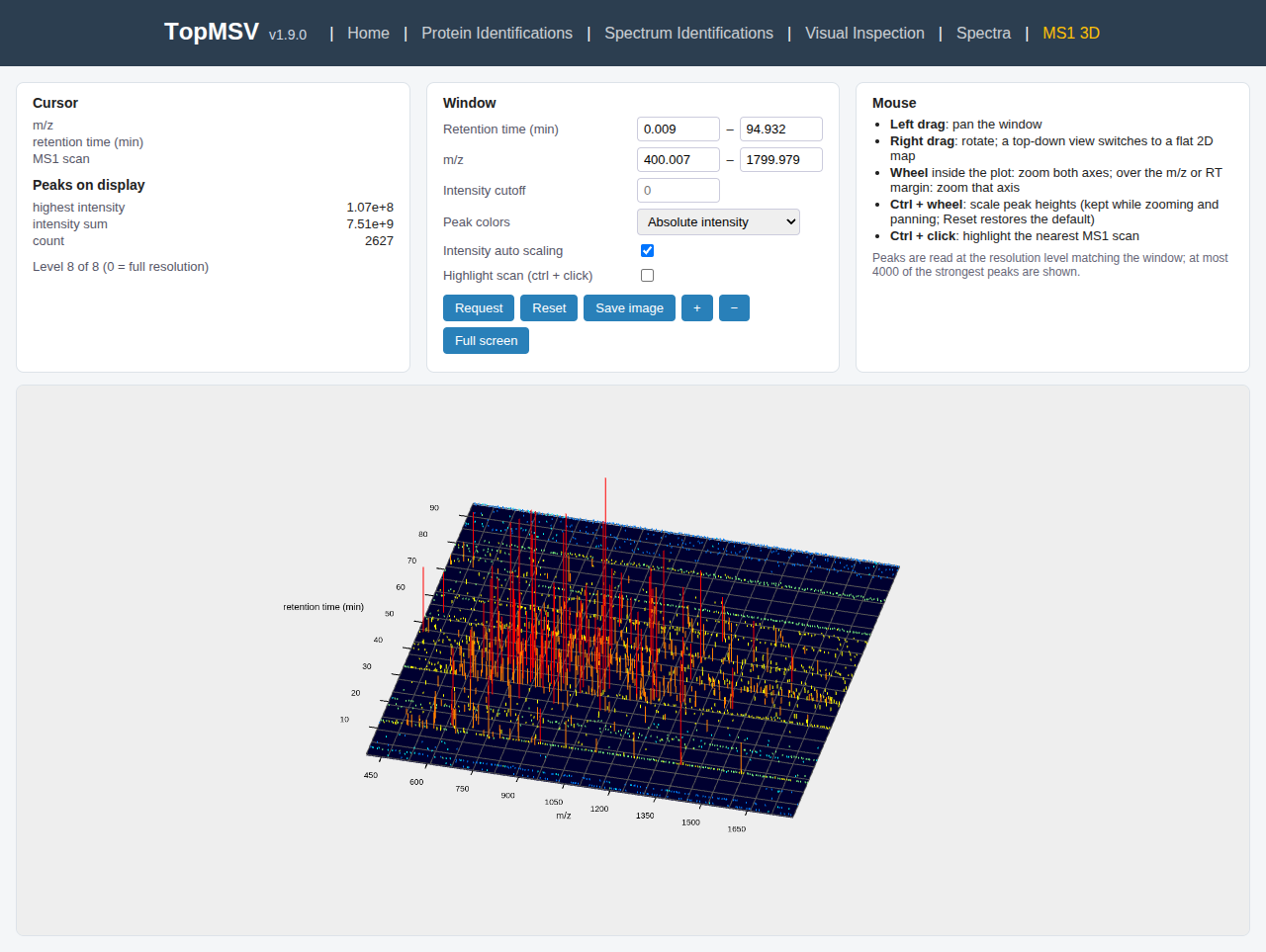
- Click "MS1 3D" in the navigation bar. The page shows the MS1 peaks of the whole LC-MS run: the x axis is the m/z value, the depth axis is the retention time, and the height of a peak is its intensity.
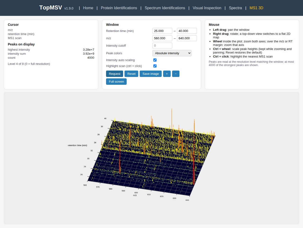
- In the "Window" panel, set the retention time range to 25 – 40 min and the m/z range to 560 – 640, check "Highlight scan", and click "Request". The window around the precursor of scan 876 (retention time 29.8 min, m/z 572) is shown at a higher resolution.
- Drag the plot with the left mouse button to pan, use the mouse wheel to zoom, hold Ctrl and use the mouse wheel to scale the peak heights, and drag with the right mouse button to rotate the view. Hold Ctrl and click a peak to highlight its MS1 scan. Click "Save image" to save the plot as a PNG file.